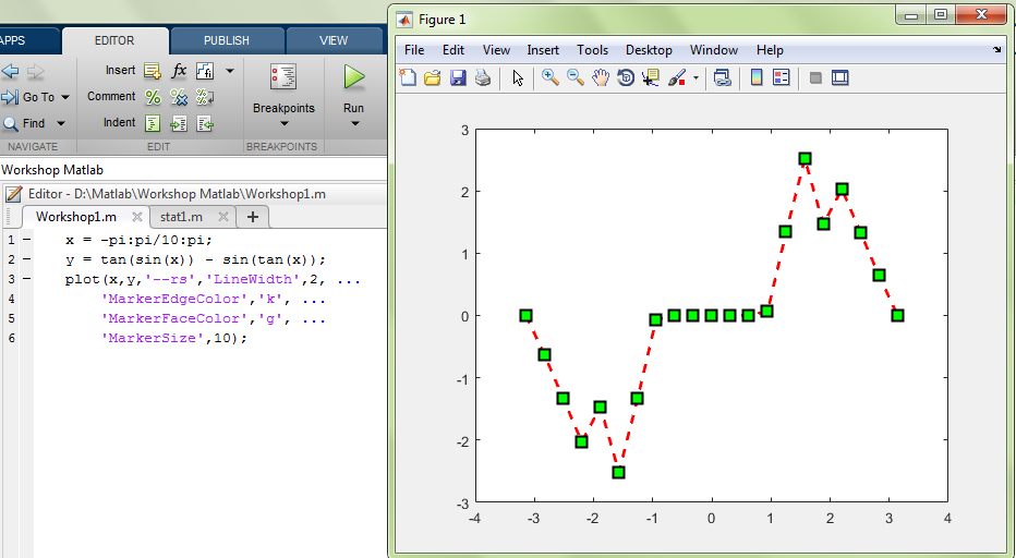
This chapter will explain common plot function in Matlab. To draw graphics in Matlab we can use plot() function as defined below:
Syntax :
x = -pi:pi/10:pi;
y = tan(sin(x)) – sin(tan(x));
plot(x,y,’–rs’,’LineWidth’,2, ‘MarkerEdgeColor’,’k’, ‘MarkerFaceColor’,’g’, ‘MarkerSize’,10);
Where :
x is the axis range
y is the result
‘–rs’ is the line model which is double strip –, “r” for red color and “s” for square marker
‘LineWidth’ determines the line width which is 2
‘MarkerEdgeColor’ determines the marker edge color which is ‘k’ for black color
‘MarkerFaceColor’ determines the marker face color which is ‘g’ for green color
‘MarkerSize’ determines the marker size which is 10
Result :
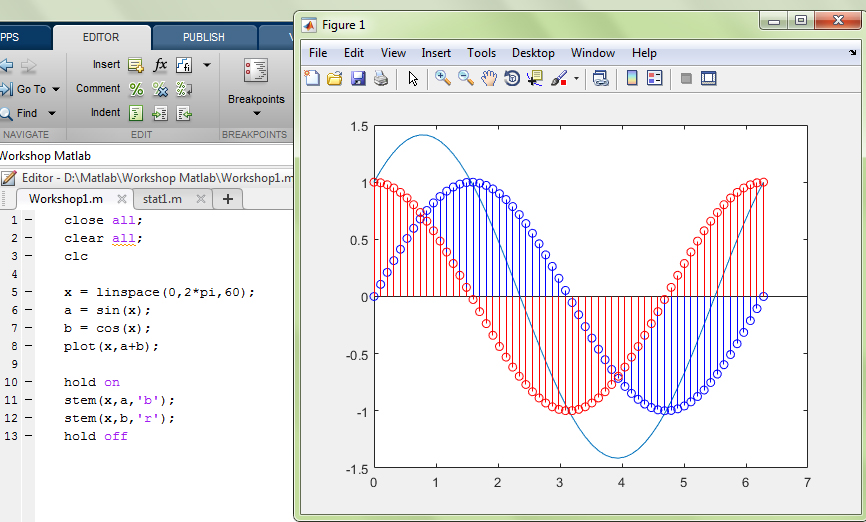
To add two graphics in Matlab we can use plot() function followed by hold on and hold off as defined below:
Syntax :
x = linspace(0,2*pi,60);
a = sin(x);
b = cos(x);
plot(x,a+b);
hold on
stem(x,a,’b’);
stem(x,b,’r’);
hold off
Result :
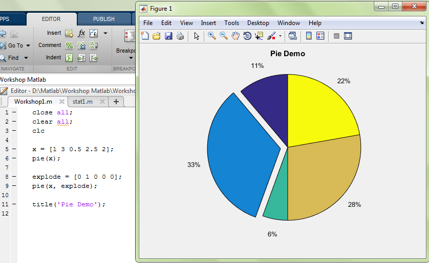
To add title and axis label we can use title() and axes([xmin xmax ymin ymax])
Syntax :
x = [1 3 0.5 2.5 2];
pie(x);
explode = [0 1 0 0 0];
pie(x, explode);
title(‘Pie Demo’);
Result :
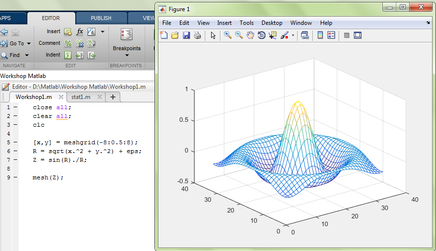
To draw 3D graphics we can use meshgrid()
Syntax :
[x,y] = meshgrid(-8:0.5:8);
R = sqrt(x.^2 + y.^2) + eps;
Z = sin(R)./R;
mesh(Z);
Result :
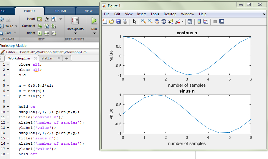
To show some graphics in one figure we can use subplot() function
Syntax :
n = 0:0.5:2*pi;
x = cos(n);
y = sin(n);
hold on
subplot(2,1,1); plot(n,x);
title(‘cosinus n’);
xlabel(‘number of samples’);
ylabel(‘value’);
subplot(2,1,2); plot(n,y);
title(‘sinus n’);
xlabel(‘number of samples’);
ylabel(‘value’);
hold off
Result :